From Detection to Topology: Mapping Red Deer Trail Networks from Airborne LiDAR

Background

The Oostvaardersplassen (OVP) is one of the most unusual nature reserves in the Netherlands. Located in the Flevoland polder — land reclaimed from the IJsselmeer in the 1960s — it was originally intended for industrial use. But before any development began, reed (Phragmites australis) colonised the wet, flat terrain, and birds followed. The site was eventually designated a nature reserve, and in 1992 red deer (Cervus elaphus) were introduced to the 36 km² marsh.

Over the following decades, the deer left a lasting mark on the landscape. Moving daily between the open grassland border zone and the dense reedbeds — for shelter, rest, and grazing — they trampled the vegetation into a dense network of trails. These trails are not random scratches; they are persistent, heavily used corridors that structurally alter the reed canopy and shape the spatial ecology of the marsh.

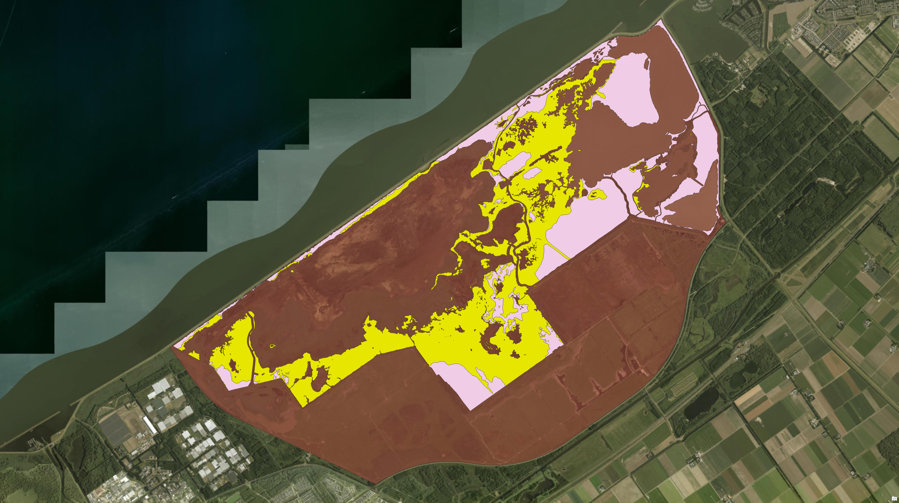
The Oostvaardersplassen. Dark red zone indicate the boundary of the Oostvaardersplassen. Yellow and pink zones indicate the reedbed marsh areas.

The Published Foundation

In a recently published study (Wang et al., 2025, Frontiers in Remote Sensing), we presented a four-step workflow to detect and map these trails from airborne laser scanning (ALS) point clouds acquired by the Dutch national survey programme (AHN).

The core idea is that deer trails compress vegetation downward, creating subtle depressions in the 3D point cloud. The workflow:

1. Pre-processing — Re-tiling, spatial clipping, and statistical outlier removal of a 42.3 GB dataset.
2. Near-terrain filtering — Iterative 3D grid subdivision to isolate ground-level returns from reed canopy.
3. DTM generation — Inverse Distance Weighting interpolation at 10 cm resolution.
4. Trail extraction — Iterative Laplacian smoothing to amplify depression signatures, followed by 3D structure tensor voting to confirm elongated linear features.

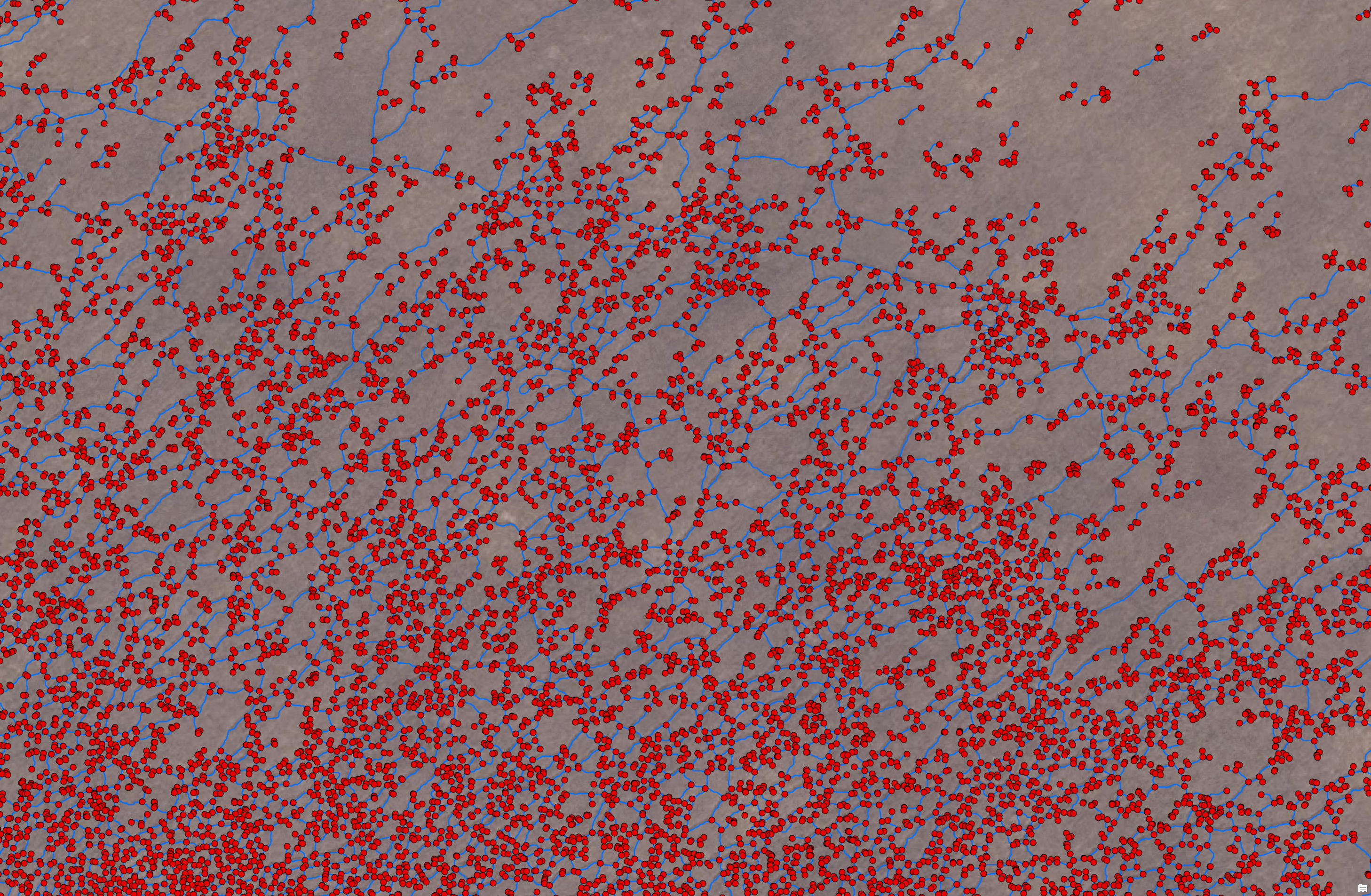
The result was a trail map covering 1.88 km² (11.6% of the study area), validated against manually digitised reference data with an overall accuracy of 93% in red deer-only areas and 90% in mixed red deer/goose grazing zones.

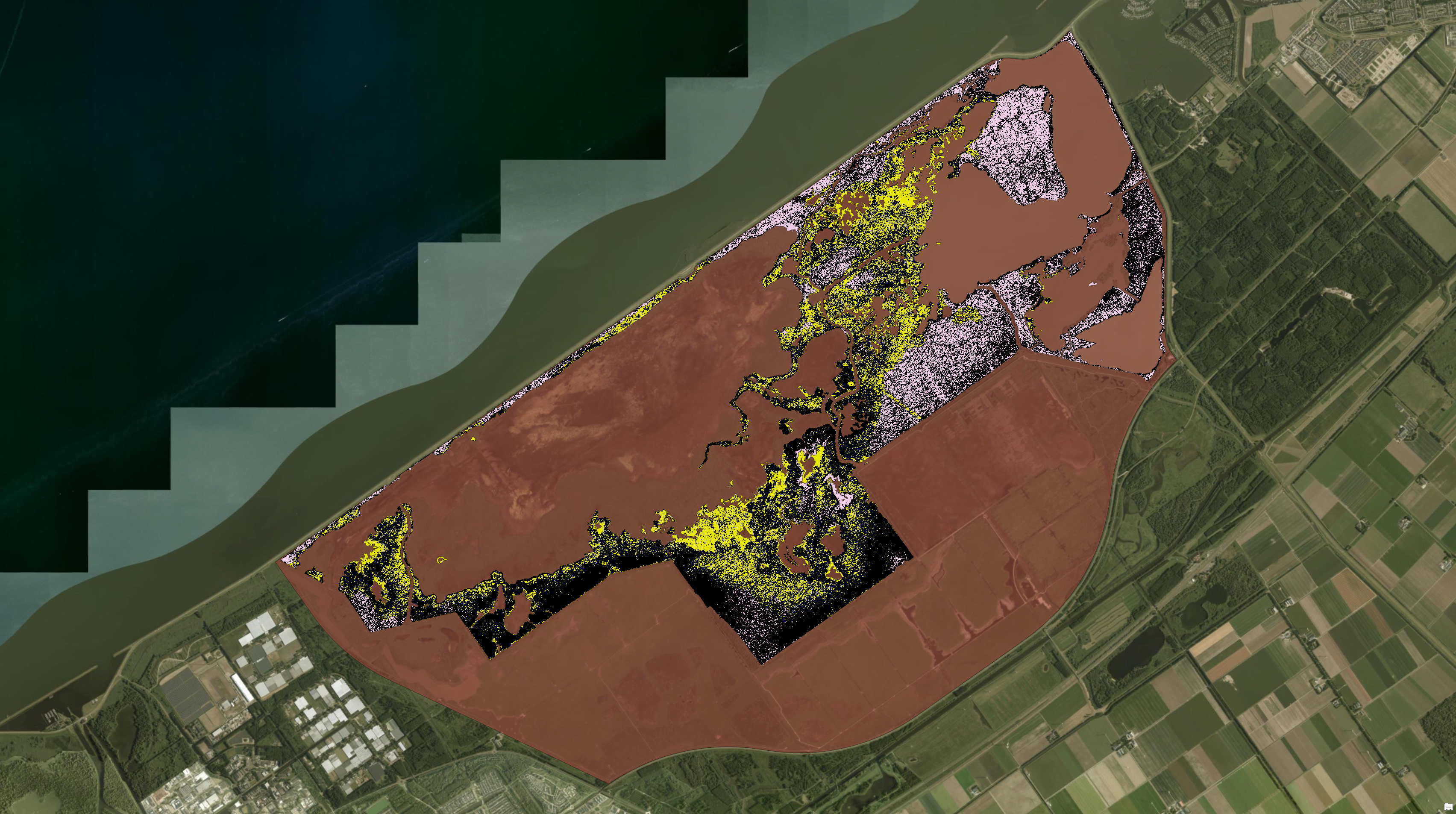
Extracted trails overlaid on the studied reedbed marsh area in OVP. The concentration of trails at the grassland–reedbed boundary and along internal drainage channels is clearly visible in this image.

What Comes Next: Centerlines and a Trail Graph

The published workflow outputs sets of grids, however, it leaves the trail network as a volumetric mass of points or grids, not a geometric structure ecologists can analyse.

The natural next step is to ask: what does the connectivity of these trails actually look like?

To answer that, I processed the extracted trail grids through two further stages:

1. Centerline extraction — reducing the width of each trail to its medial axis, a single-pixel-wide skeleton.
2. Graph construction — converting the skeleton into a proper topological graph with nodes (junctions and endpoints) and edges (trail segments), which is now a true linear feature representation of the OVP marsh.

The rest of this post documents the methodology behind both stages.

Stage 1 — Centerline Extraction

Discretization

The input is a set of unordered 3D grids P = {p₁, p₂, …, pₙ}, where pᵢ = (xᵢ, yᵢ, zᵢ) ∈ ℝ³. To apply morphological operations, the XY projection is rasterized into a binary grid I : Ω → {0,1}, where Ω ⊂ ℤ². The mapping from real coordinates to grid indices at resolution δ (set to 0.1 m, matching the resolution of the output) is:

c = (x − x_min) / δ
r = (y_max − y) / δ

The grid cell is set to 1 if any point maps into it, otherwise 0.

Morphological Closing

The extracted trail points are often sparse — the ALS returns are not uniformly distributed, and short gaps appear in the binary grid. To produce a coherent surface before skeletonization, morphological closing is applied using a disk structuring element B of radius R (variable closing_radius, set to 4 pixels = 0.4 m):

A ∙ B = (A ⊕ B) ⊖ B

Dilation (⊕) expands the trail boundary, bridging gaps smaller than 2R = 0.8 m. Erosion (⊖) then retracts the boundary back, restoring approximate width while preserving the connectivity established by dilation.

Skeletonization

The medial axis transform extracts the skeletal subset S ⊆ A — the locus of centres of all maximal disks inscribed in the closed shape A. Conceptually, every point on the skeleton is equidistant from two or more boundaries of the shape, making it the geometric “spine” of the trail. The Lee (1994) algorithm is used (skimage.morphology.skeletonize), which guarantees an 8-connected, one-pixel-wide output.

3D Reconstruction

Skeletonization operates in 2D and discards elevation. To recover Z, a KD-tree (scipy.spatial.cKDTree) is built over the XY coordinates of the original input points. Each skeleton pixel is assigned the elevation of its nearest neighbour in the original cloud:

z_node = z of argmin_{p ∈ P} ‖(p_x, p_y) − (x_g, y_g)‖₂

The output of this stage is a set of 3D centerline points exported as LAZ, GeoTIFF, and ESRI Shapefile.

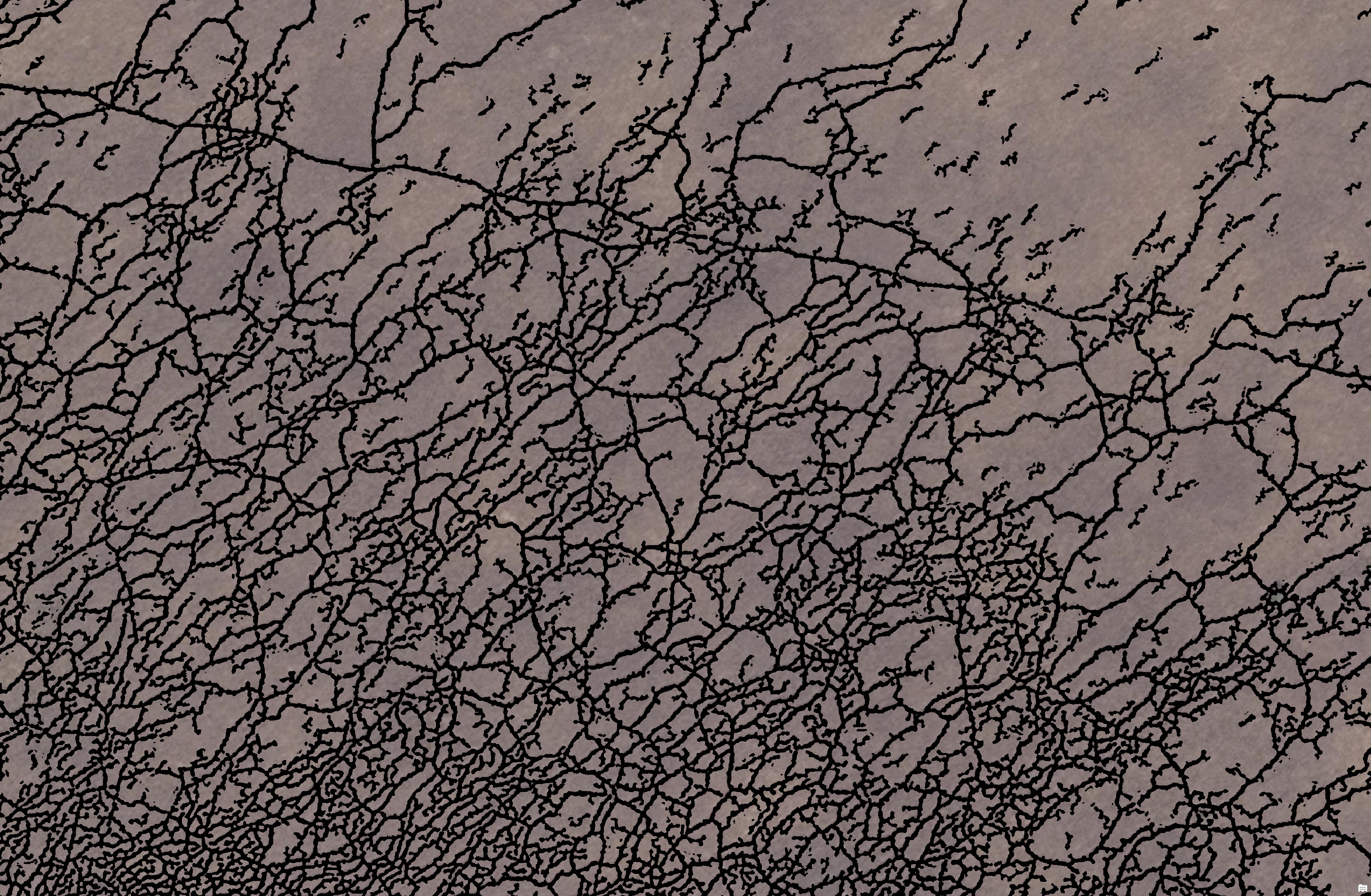
Red deer trails extracted from the AHN4 point clouds, which is the output of the publication.

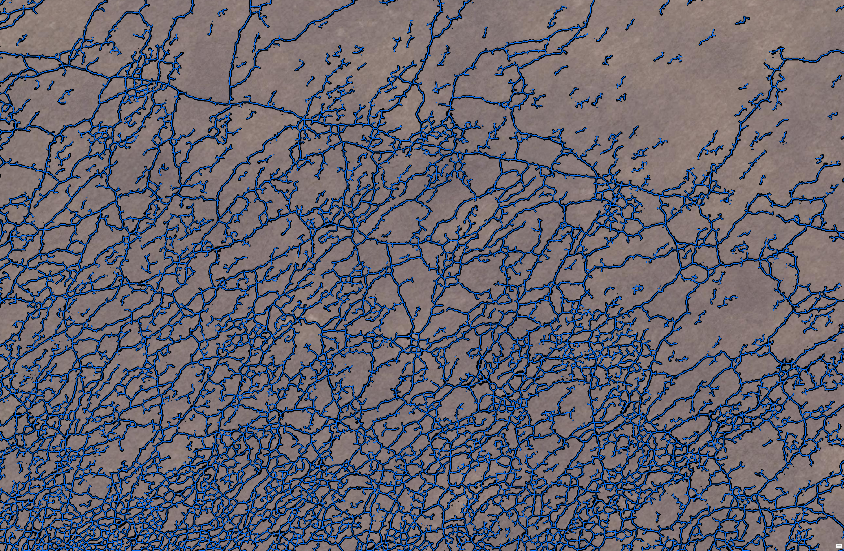
The same centerlines rendered as vector polylines (blue) in GIS. The dense branching pattern mirrors the complexity of the trail network in the reedbed marsh area.

Stage 2 — Graph Construction and Topology Cleaning

The second script takes the centerline point clouds as input and constructs a proper topological graph.

Graph from Skeleton

The binary skeleton S is converted into an undirected graph G = (V, E):

• Nodes V: every skeleton pixel becomes a node.
• Edges E: two nodes are connected if they are 8-connected neighbours (horizontal, vertical, or diagonal). Diagonal edges are weighted by √2 · δ ≈ 0.141 m to reflect true Euclidean distance.

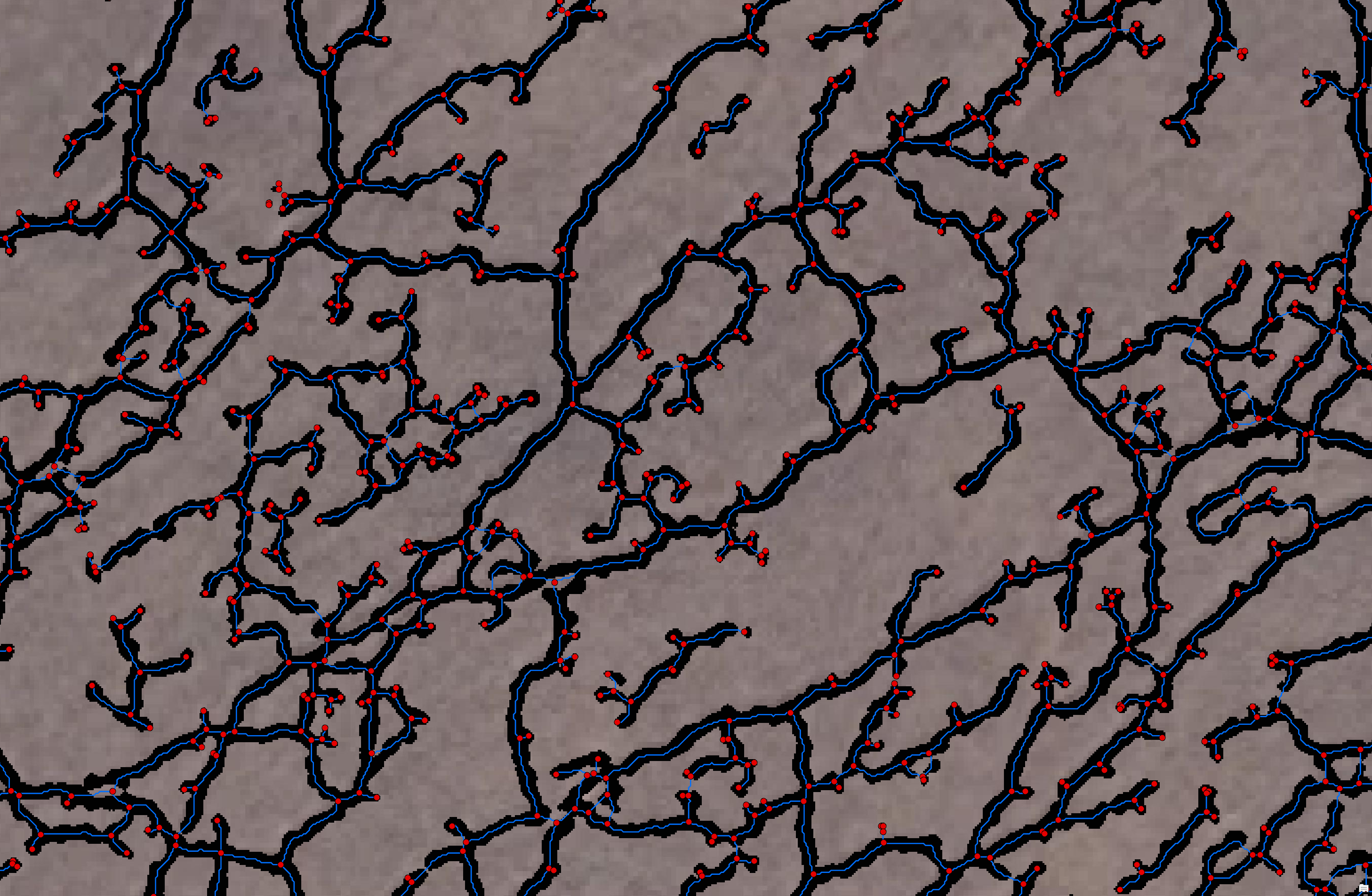
At this raw stage, the graph has one node per skeleton pixel — tens of thousands of nodes per tile — as visible below.

The constructed graph based on the extracted centerlines: red dots are nodes, blue lines are edges.

Topology Cleaning

The raw skeleton graph contains two types of artefacts introduced by the discrete rasterization:

Cycle contraction. Small loops (perimeter < max_cycle_len = 20 pixels = 2 m) arise from rasterization bubbles where a trail slightly widens. For each small cycle Cₖ, all its nodes are contracted into a single centroid node:

v_centroid = (1/|Cₖ|) · Σ_{v ∈ Cₖ} v

Junction merging. At a real intersection (T or + shape), multiple adjacent pixels have degree > 2. These are not distinct junctions — they are one physical crossing represented by a cluster of nodes. Connected components of high-degree nodes are identified and contracted into a single centroid node per component.

After cleaning, only meaningful nodes remain: junctions (degree ≥ 3), endpoints (degree 1), and bridge nodes at tile boundaries. The definitions of the Nodes and Edges of the graph are therefore updated as:

• Nodes V’ : topologically significant points only: junctions (degree ≥ 3, where trails fork or converge), endpoints (degree 1, trail dead-ends), and bridge nodes (endpoints snapped to a tile boundary, flagged is_bridge = 1 for inter-tile stitching). All intermediate degree-2 pixels are no longer represented as nodes.
• Edges E’ : each edge is now a polyline encoding the full 3D geometry of a trail segment between two consecutive meaningful nodes. The intermediate degree-2 skeleton pixels are dissolved into the edge’s coordinate sequence, preserving the curvature of the trail path without bloating the node count.

Close-up of the same graph. Each red node represents a topologically significant location — a trail fork, a merge point, or a dead end. Each edge encodes a trail segment with full 3D geometry.

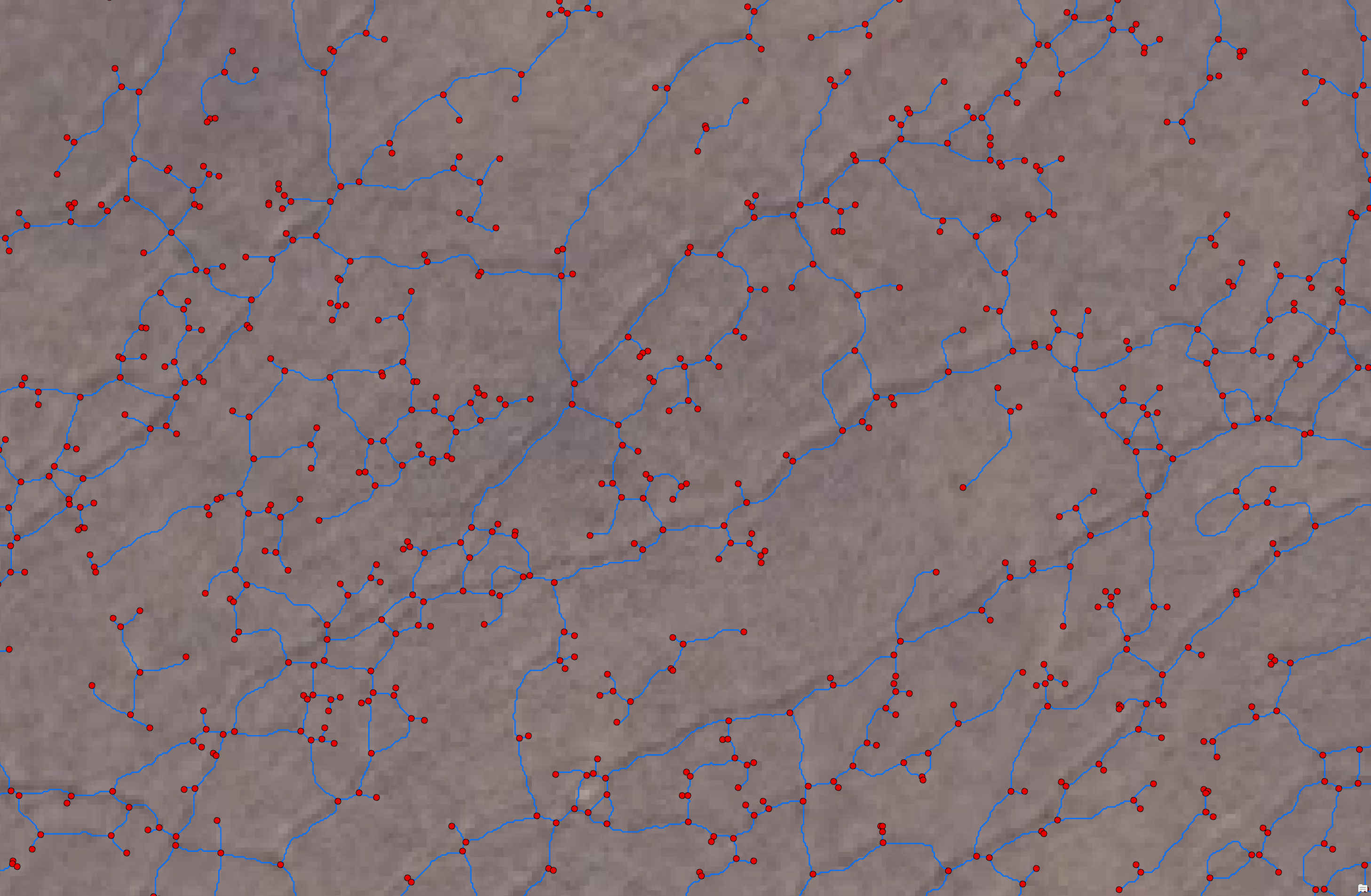
The topology graph at area scale without extracted trail clusters. Red nodes mark junctions and endpoints; blue lines are trail segments (edges). The structure clearly reflects the branching pattern of deer movement corridors.

Boundary Snapping

Because the input data is processed tile by tile, trail segments crossing a tile boundary are terminated at the tile edge. Any endpoint whose real-world distance to the tile boundary falls within a configurable threshold (BOUNDARY_THRESH = 0.2 m) is snapped to the exact boundary coordinate and flagged as a bridge node (attribute is_bridge = 1). This ensures that adjacent tiles stitch together cleanly during downstream network assembly.

Output

Each processed tile produces:

• Nodes shapefile — point geometry at every junction, endpoint, and bridge node, with is_bridge and node_id attributes.
• Edges shapefile — polyline geometry for every trail segment between nodes, with embedded 3D coordinates.
• GeoTIFF — the binary skeleton raster.
• LAZ — the 3D centerline point cloud.

Implementation

Both scripts are written in Python 3, with the following key dependencies:

Both scripts use a ProcessPoolExecutor to saturate available CPU cores across tiles. Script 2 additionally accelerates the rasterization and morphological closing steps on GPU via CuPy, which significantly reduces per-tile processing time for large datasets.

The two Python scripts can be viewed here: 1_extract_centerlines_v4.py — centerline extraction  |  2_convert_to_graph_v1_1_3_5.1.py — graph construction

The core of Script 1 is the per-tile worker: rasterize → close → skeletonize → recover Z via KD-tree:

closed_grid = binary_closing(grid > 0, disk(closing_radius))
skeleton    = skeletonize(closed_grid)

tree    = cKDTree(points_xyz[:, :2])
_, idxs = tree.query(np.vstack((skel_x, skel_y)).T, k=1)
skel_z  = points_xyz[idxs, 2]

Script 2 adds GPU-accelerated rasterization (CuPy) and the topology-cleaning loop that contracts small cycles and merges adjacent junction clusters:

# GPU rasterization
gpu_grid   = cp.zeros((height, width), dtype=cp.uint8)
gpu_grid[idx_y, idx_x] = 1
gpu_closed = ndimage.binary_closing(gpu_padded, structure=cp.asarray(disk(closing_radius)))

# Cycle contraction
for cycle in nx.minimum_cycle_basis(G):
    if len(cycle) < max_cycle_len:
        nx.contracted_nodes(G, centroid_node, *cycle[1:], copy=False)

What the Graph Enables

Representing the OVP trail network as a proper graph opens up a range of analyses that are not possible from raw point clouds or raster masks:

• Network connectivity — identify isolated trail components versus the main connected network.
• Trail segment lengths — compute edge weights (Euclidean length along the polyline) to characterise movement corridor distances.
• Junction topology — degree distribution of nodes reveals how many trails converge at each intersection, which may correlate with deer traffic intensity.
• Shortest paths — measure least-cost movement routes between grassland entry points and interior resting areas.
• Graph simplification — aggregate short edges to produce a coarser, human-readable network for visualisation.

The graph is stored in a standard GIS format (separate nodes and edges shapefiles in EPSG:28992 — the Dutch national coordinate system), so it can be loaded directly into QGIS, ArcGIS, or any Python-based network analysis library.

Next Steps

The per-tile graphs have been stitched into a single reserve-wide network by matching bridge nodes at shared tile boundaries — each flagged endpoint is aligned to its counterpart in the adjacent tile, and the edges are joined to form a continuous graph spanning the full OVP marsh. The resulting network is a complete linear feature representation of all detected red deer trails across the reserve.

With that foundation in place, several directions become possible:

Movement behaviour analysis. Graph centrality measures — in particular betweenness centrality — can identify which trail segments carry the most network traffic, i.e. which corridors are the most critical connectors between distant parts of the reserve. Degree distribution at junctions reveals whether the network has a few high-traffic hubs or a more uniform branching structure. Shortest-path routing between the grassland entry points and interior resting areas can approximate the preferred daily movement routes of the deer.

Ecological interpretation. Trail density and network complexity are proxies for cumulative grazing pressure: areas with a denser, more interconnected graph have experienced more intensive trampling over time. This can be cross-referenced with vegetation maps to quantify how trails have fragmented the reed canopy into patches, creating edge habitats that may favour different plant communities or waterbird species. The network also provides spatial context for interpreting biomass loss and reed structure degradation observed in field surveys.

Temporal monitoring. The AHN dataset is periodically re-acquired. Repeating the extraction workflow on a later acquisition and comparing the resulting graphs — measuring added or removed edges, changes in connectivity, shifts in trail density — would provide a quantitative record of how the trail network has evolved following the deer population management measures introduced in 2018.

Transferability. The methodology is not specific to red deer or to the OVP. Applying the same pipeline to other wetland reserves, other ungulate species (roe deer, elk, wild boar), or other high-resolution ALS datasets would test the robustness of the approach and broaden its ecological relevance. The graph representation is also generalisable to other types of linear landscape features — hedgerows, drainage ditches, or stone walls — that leave a topographic signature detectable in dense point clouds.

Integration with agent-based models. The trail graph is a natural input for agent-based simulations of animal movement. Nodes become waypoints; edge weights encode traversal cost; the full network defines the space of possible paths. Calibrating such a model against GPS collar data, where available, could help disentangle which aspects of trail structure are driven by individual preference versus herd-level path reinforcement.